A few years ago, Peter Norvig published a simple economic simulation that models the pace of wealth inequality. The basic premise is this: there is a population of actors, each with a preset wealth level. The economy is driven by transactions in which two actors will randomly exchange a random amount of their wealth:
def transaction(a, b):
    s = a + b
    r = np.random.uniform(0, s)
    return r, s - r
So for a given input:
In: transaction(100, 100)
Out: (79.90256295428071, 120.09743704571929)
Ultimately, the idea is that the economy will stabilize around some level of distributed wealth. We can measure the resulting level of wealth inequality using the popular Gini coefficient. A value of 0% on this scale means perfect income equality, while a value of 100% means all of the wealth belongs to one individual. For reference, here are the Gini coefficients for income in a few countries over the last few decades (source: OECD). Note that the Gini coefficient for actual wealth is higher in many of these countries:
| Country | 1970s | 1980s | ~1990 | 1990s | ~2000 | 2000s | ~2010 |
|---|---|---|---|---|---|---|---|
| Mexico | 0.452 | 0.519 | 0.507 | 0.474 | 0.476 | ||
| Turkey | 0.434 | 0.49 | 0.43 | 0.409 | |||
| Chile | 0.427 | 0.403 | 0.394 | ||||
| Portugal | 0.354 | 0.329 | 0.359 | 0.356 | 0.385 | 0.353 | |
| United States | 0.316 | 0.337 | 0.348 | 0.361 | 0.357 | 0.38 | 0.378 |
| Israel | 0.326 | 0.329 | 0.338 | 0.347 | 0.378 | 0.371 | |
| Greece | 0.413 | 0.336 | 0.336 | 0.345 | 0.321 | 0.307 | |
| Spain | 0.371 | 0.337 | 0.343 | 0.342 | 0.319 | 0.317 | |
| Estonia | 0.349 | 0.315 | |||||
| Italy | 0.309 | 0.297 | 0.348 | 0.343 | 0.352 | 0.337 | |
| United Kingdom | 0.268 | 0.309 | 0.354 | 0.336 | 0.351 | 0.331 | 0.345 |
The coefficient is typically calculated as the proportional area between the Lorenz curve (which plots income across the population) and a 45° line indicating perfect equality, or half the mean absolute difference, but can be alternately simplified as follows:

Shamelessly borrowing from Norvig's implementation, we can write this formula in Python for a given array y as:
def gini(y):
    y = sorted(y)
    n = len(y)
    numer = 2 * sum((i + 1) * y[i] for i in range(n))
    denom = n * sum(y)
    return (numer / denom) - (n + 1) / n
At first, I set out to reimplement his results in a self-contained class which you can check out in this gist: norvig.py
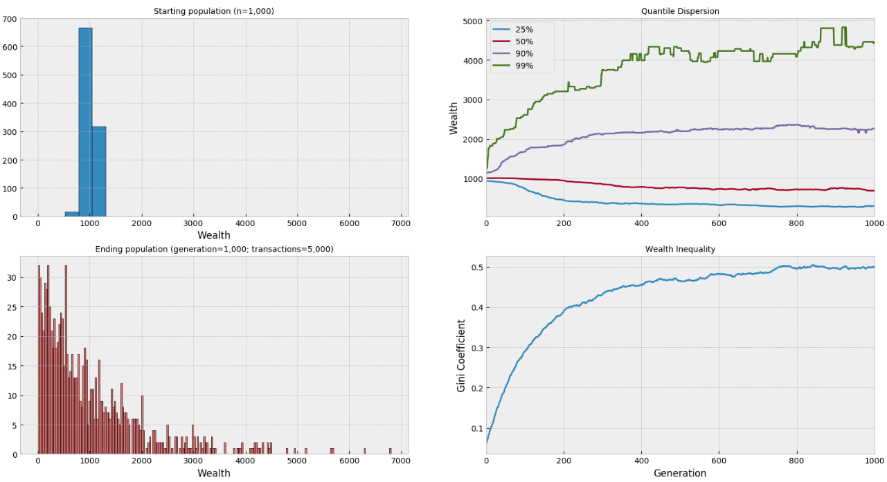
Using this class structure, we can simply simulate results using any starting population: in this case we'll generate a normally distributed population of 1,000 actors with mean 1,000 wealth units and standard deviation of 100 for a global money supply of ~1,000,000 units. We then run simulate() for 1,000 generations where 5 random transactions occur in each generation:
N = 10 ** 3
P = np.random.normal(loc=1000, scale=100, size=N)
Economy(P).simulate(10 ** 3, 5)
| generation | cum events | n | Gini | median | stdev | min | 25% | 50% | 90% | 99% | max |
|---|---|---|---|---|---|---|---|---|---|---|---|
| - | - | 1,000.00 | 0.06 | 996.42 | 100.95 | 631.43 | 931.58 | 996.42 | 1,129.26 | 1,219.62 | 1,303.34 |
| 50.00 | 250.00 | 1,000.00 | 0.20 | 996.88 | 396.02 | 4.11 | 881.93 | 996.88 | 1,467.95 | 2,225.55 | 3,199.45 |
| 100.00 | 500.00 | 1,000.00 | 0.29 | 979.90 | 543.31 | 2.38 | 729.72 | 979.90 | 1,671.62 | 2,604.19 | 4,470.64 |
| 150.00 | 750.00 | 1,000.00 | 0.35 | 959.77 | 651.84 | 2.38 | 545.36 | 959.77 | 1,791.51 | 3,103.45 | 4,470.64 |
| ··· | |||||||||||
| 850.00 | 4,250.00 | 1,000.00 | 0.50 | 713.64 | 1,003.73 | 2.21 | 279.77 | 713.64 | 2,257.96 | 4,374.45 | 7,971.72 |
| 900.00 | 4,500.00 | 1,000.00 | 0.50 | 746.12 | 982.12 | 1.29 | 273.31 | 746.12 | 2,248.29 | 4,378.17 | 6,798.36 |
| 950.00 | 4,750.00 | 1,000.00 | 0.49 | 727.84 | 974.27 | 1.29 | 277.80 | 727.84 | 2,254.34 | 4,285.54 | 6,798.36 |
| 1,000.00 | 5,000.00 | 1,000.00 | 0.50 | 678.01 | 992.68 | 1.29 | 296.12 | 678.01 | 2,257.96 | 4,440.25 | 6,798.36 |
We can also test with an alternate starting population where all actors begin with 1,000 units. Unsurprisingly, the results are the same:
P = np.array([1000] * N)
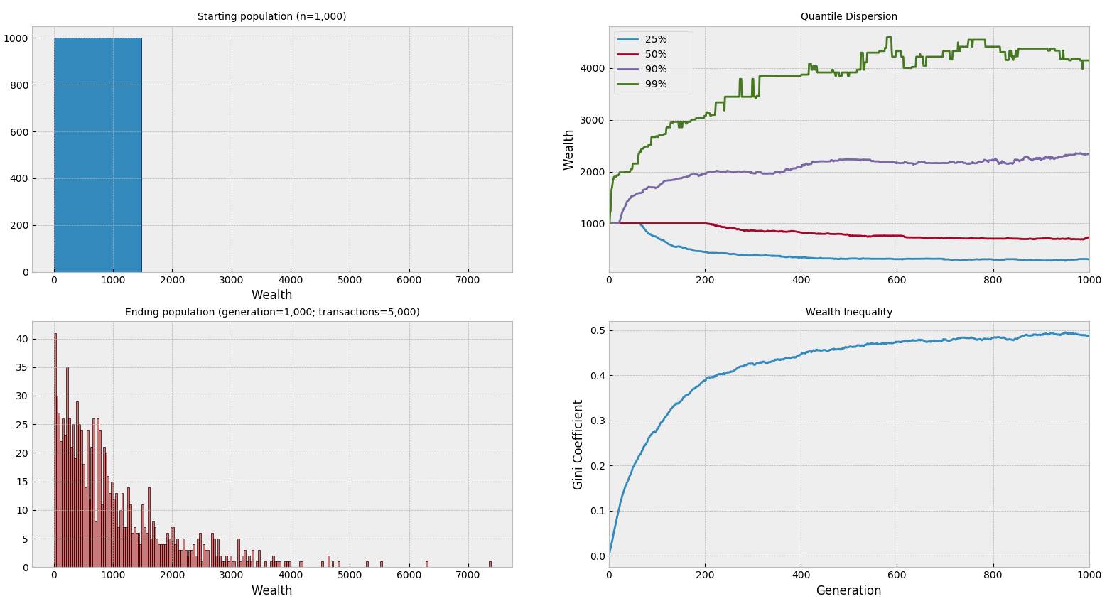
Consistent with Norvig's findings, this simple economy stablizes with an extraordinary amount of inequality where most of the population is concentrated around the lowest levels of wealth, and each transaction rapidly produces "winners" and "losers" in the market. Without any other components to redistribute wealth, this transaction model highly favors wealthy actors. But what would happen if we introduced intermediary nodes into the simulation?
Adding companies into the mix
I was curious to see an expanded model that could account for companies that receive revenue and distribute profits. I added a new "corporation" entity to the class and modified the transaction function. Before the first generation, we randomly assign all of the actors to be "employed" by a corporation:
import networkx as nx

# Using a multi-directional network graph so actors/companies can participate in multiple transactions and we can track the direction of virtual dollars
self.G = nx.MultiDiGraph()
# Add population nodes
self.G.add_nodes_from(self.population.keys(), bipartite=0)
self.G.add_nodes_from(self.corporations.keys(), bipartite=1)

# Randomly assign actors to work for each company
for cid in self.corps.keys():
    # Equal number of people work for each company
    eids = random.sample(self.population.keys(), int(len(self.population)/len(self.corps)))
    for eid in eids:
        # We add an edge in our network for each employee - eventually we'll track their earnings over time.
        self.G.add_edge(cid, eid)
In each transaction, an individual transfers a random amount of their wealth to a company - actors no longer exchange directly with one another.
def transaction(self, a, c):
    w = self.population[a]
    # Actor spends a random quantity of their wealth with the company
    r = np.random.uniform(0, self.population[a])
    return w - r, self.corps[c] + r
At the end of each generation, all companies distribute 100% of their revenue randomly to their employees:
def distribute(self, cid, revenue, pop):
    while revenue > 1:
        for eid in self.G[cid].keys():
            pay = np.random.uniform(0, revenue)
            # Give rounding error to this employee:
            pay = revenue if pay < 1 else pay
            pop[0][eid] += pay
            pop[1][cid] -= pay
            revenue -= pay
    return pop
This model doesn't favor individuals with high wealth since the recipients' wealth (i.e. the employees) is not considered in the equation - a high wealth actor is free to spend any amount of money with any company and that money will always be independently distributed between its employees. As a result, we attain relative improvement: norvig.py:c197f7
N_P = 10 ** 3
N_C = 500
P = list(np.random.normal(loc=1000, scale=100, size=N_P))
sim = Economy(P, N_C)
sim.simulate(10 ** 3, 20_000)
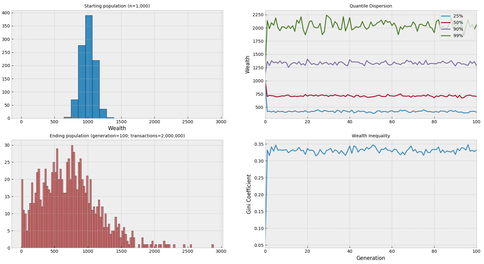
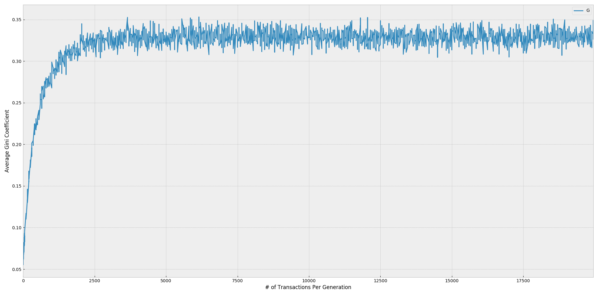
Notice in the preceding simulation we're running many more transactions in each generation than before, and the stable level of inequality is reached after the first generation - since companies redistribute their revenue at the end of the period, the model is highly sensitive to the number of transactions occurring beforehand. The level shown above appears to be the limit, while faster distribution (i.e. fewer transactions per generation) leads to less overall movement in the population from the starting level of wealth.
Additionally, there are still many simplistic assumptions in this revised model:
- There is no concept of exchange of value or price, allowing a wealthy actor to distribute a high percent of their wealth to a random company in a single transaction.
- Actors have no self-preserving tendencies - a wealthy actor should prefer to remain wealthy and spend a smaller proportion of their wealth.
- Companies are not able to hire or fire employees when they have excess/deficient revenue. Similarly, actors can't quit if they aren't paid sufficiently.